When you finished reading part 1 of the introduction you might have wondered how to draw more than one line or curve into on plot. I will show you now.
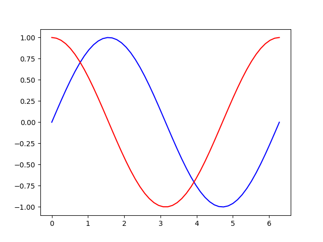
To make it a bit more interesting we generate two functions: sine and cosine. We generate our x-values with numpy’s linspace function
import numpy as np
import matplotlib.pyplot as plt

x = np.linspace(0, 2*np.pi)
sin = np.sin(x)
cos = np.cos(x)
plt.plot(x, sin, color='b')
plt.plot(x, cos, color='r')
plt.show()
You can plot two or more curves by repeatedly calling the plot method.
That’s fine as long as the individual plots share the same axis-description and values.
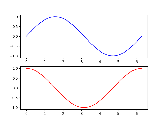
Subplots
fig = plt.figure()
p1 = fig.add_subplot(2, 1, 1)
p2 = fig.add_subplot(2, 1, 2)
p1.plot(x, sin, c='b')
p2.plot(x, cos, c='r'
The add_subplot method allows us to put many plots into one “parent” plot aka figure. The arguments are (number_of_rows, number_of_columns, place in the matrix) So in this example we have 2 rows in 1 column, sine is in first, cosine in second position:
when you have a 2 by 2 matrix it is counted from columns to row
fig = plt.figure()
p1 = fig.add_subplot(221)
p2 = fig.add_subplot(222)
p3 = fig.add_subplot(223)
p4 = fig.add_subplot(224)
p1.plot(x, sin, c='b')
p2.plot(x, cos, c='r')
p3.plot(x, -sin, c='g')
p4.plot(x, -cos, c='y')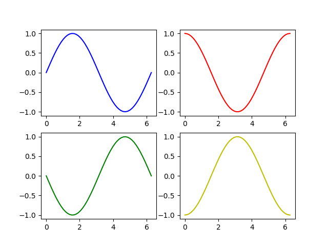
The code is available as a Jupyter Notebook on my github
More about matplotlib in Part 3